


Next: 天体の個数密度
Up: 密度揺らぎの統計的性質
Previous: 密度揺らぎの smoothing
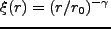
揺らぎの二体相関関数は
 |
(4.138) |
で定義される。ここで等方性より
 とした。これは距離
 離れた点での揺らぎの値がどれだけ相関しているかを示す量である。この
 を Fourier 変換すると、
 |
(4.139) |
となり、 が power spectrum
 の Fourier 変換になっていることがわかる。
なお、本当は smoothing された field での二体相関関数であるため  に
対して window function
に
対して window function
 を掛けて積分する必要があるが、
 より角度積分によって
 となり、
また
となり、
また のため、こちらの cut-off の方が重要であり、smoothing は本質的
ではない。
のため、こちらの cut-off の方が重要であり、smoothing は本質的
ではない。
ここで
 と置くと、
と置くと、
 |
(4.140) |
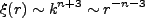
となる。観測された銀河分布では、
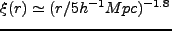 となることが知られている。従って、もし銀河と dark
matter の分布が同じならば、このスケールで、
となることが知られている。従って、もし銀河と dark
matter の分布が同じならば、このスケールで、 程度になってい
なければならない。これは CDM の予想とは大体一致する。
程度になってい
なければならない。これは CDM の予想とは大体一致する。
Figure 8:
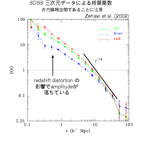 |
実際には、銀河と dark matter の分布は同じではない。それぞれの二体相関関
数を
 と書き、
と書き、
 |
(4.141) |
と置く。この は bias parameter と呼ばれる。は原理的にはスケール、時
間に依存するが、簡単に定数とすることが多い。
は bias parameter と呼ばれる。は原理的にはスケール、時
間に依存するが、簡単に定数とすることが多い。
Figure 9:
 |
ここでが1になるスケールを考える。つまり、
 と置いた場合の
 である。これはの
amplitude の指標になっている。dark matter を考えると、線型(でE-dS)の場合、
である。これはの
amplitude の指標になっている。dark matter を考えると、線型(でE-dS)の場合、
 であるから、
 |
(4.142) |
となる。そこで、実際に観測される銀河の相関関数のが と共にどう進
化するかを見れば、これは銀河形成を理解するためのよい指標になる。high-
での相関関数はまだ観測がはじまったばかりであるが、観測は予想される dark
matter のよりも大きい値を示唆している。
と共にどう進
化するかを見れば、これは銀河形成を理解するためのよい指標になる。high-
での相関関数はまだ観測がはじまったばかりであるが、観測は予想される dark
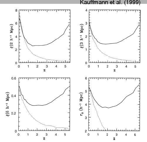
matter のよりも大きい値を示唆している。 -body simulation と準解
析的モデルの組み合わせによる解析では、が大きくなるにつれて bias が大
きくなる傾向が見られる(図11)。
-body simulation と準解
析的モデルの組み合わせによる解析では、が大きくなるにつれて bias が大
きくなる傾向が見られる(図11)。
Figure 10:
Ouchi et al. (2001)
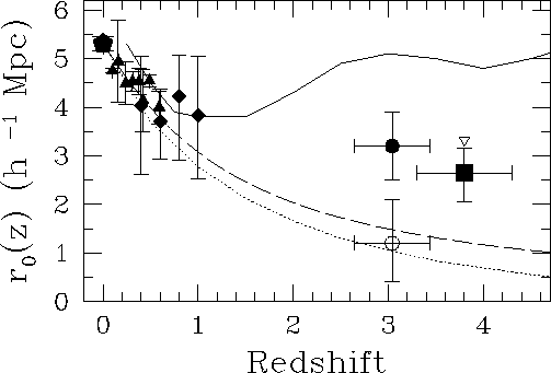 |
Figure 11:
 |
Next: 天体の個数密度
Up: 密度揺らぎの統計的性質
Previous: 密度揺らぎの smoothing
NAGASHIMA Masahiro
2009-03-12